Every trader who has ever looked at a naive gamma exposure chart knows the frustrating reality: the numbers you are looking at are from yesterday. Open interest (the foundation of every gamma exposure calculation) is settled and published after the close, available only the following morning. By the time the market opens again, the numbers are already stale. Intraday, you are flying blind.
This article describes how we approached that problem, what we built, and what we found. It is not a tutorial. It is an account of a real research and engineering project, with real results, that we believe represents a meaningful step forward in how options positioning can be monitored in real time.
What Professional Tools Currently Offer and What They Cost
A small but growing ecosystem of commercial platforms has emerged to address exactly this gap. They fall into two broad categories with meaningfully different approaches, coverage, and price points.
Category 1: Positioning and GEX Model Tools
These platforms derive gamma exposure and dealer positioning estimates from structured exchange data: primarily the Cboe Open-Close Volume Summary, which tags trades by participant type (Market Maker, institutional, retail) and direction (opening vs closing). The output is typically a set of GEX charts, gamma walls, and positioning overlays updated on a delayed intraday basis or end-of-day. Some also incorporate proprietary modelling layers on top of the raw exchange data.
| Category | Price* | Notes |
|---|---|---|
| Positioning platforms (Cboe Open-Close based) | ≈$250–$300 / month | GEX charts, gamma walls and positioning overlays derived from the Cboe Open-Close feed; some advertise direct market maker positioning across strikes and expiries. |
| Institutional-leaning data services | $700+ / month | Thousands of securities, history back a decade or more, API access. |
| Flow and GEX aggregators | ≈$50–$130 / month | Options flow and dark pool aggregation with GEX tools or modeled overlays included; instrument coverage varies. |
| Research and model shops | Not publicly listed | Daily GEX models and volatility tools. Pricing available on request. |
*Approximate list prices as of mid-2026, rounded from public pricing pages; tiers and prices change. Named examples, with rung-by-rung placement and prices, are in the GEX Data Ladder. These are illustrative examples only. The space is larger and evolving. The underlying data source for positioning tools (the Cboe Open-Close Volume Summary) is available in three tiers: an end-of-day file delivered overnight, a 10-minute interval feed, and a 1-minute interval feed delivered minutes after each interval closes. Most subscribers work from the end-of-day file. The 1-minute intraday tier, available via SFTP or Snowflake, provides a genuine near-real-time view for SPX. Only for SPX, where Cboe's exchange coverage is complete. For equities and ETFs, where Cboe captures roughly 25 to 40% of total volume, the open-close classification is structurally incomplete regardless of the update frequency purchased.
Category 2: Live Tape Aggregators
A separate class of tools takes a different approach: a handful of established tape-reading platforms (one of which was acquired outright by Cboe). These services do not wait for the delayed Open-Close file. They tap the live multi-exchange OPRA tape and apply proprietary algorithms to classify order flow in real time: distinguishing sweeps from blocks, aggressive bids from passive offers, and inferring whether large prints represent new positioning or closing flow. The result is near-instantaneous flow alerting.
The trade-off is scope. Real-time tape reading excels at surfacing large individual prints as they happen, but it does not reconstruct a continuous, strike-level OI surface. It answers "something large just traded here." It does not answer "what does aggregate positioning look like across all strikes right now." The two approaches are complementary rather than equivalent.
What Makes This Approach Different
The tools above show you flow: who opened or closed what volume, in which direction, categorised by actor type. That is genuinely useful. What this model produces is something different: a reconstruction of the OI surface itself: how many contracts are estimated to be outstanding at each strike right now, built up incrementally from a trained model applied to every 15-minute bar of the session. One is a signal about events as they occur; the other is a continuously updated picture of the accumulated positioning.
There is also a subtlety in the "real-time" framing of 1-minute CBOE data that is worth understanding. When a large order hits a market maker, their delta hedge is executed instantaneously (within milliseconds of the fill). The Cboe Open-Close classification of that trade arrives a few minutes later at best: the interval must close and the file must be compiled and delivered. By the time the positioning data reaches a subscriber's screen, the hedging flow is already in the price. Our model is not faster at detecting individual events. What it offers instead is the cumulative view: where has OI been building or unwinding across the session as a whole, and what does that imply for where gamma pressure is concentrated right now.
This cumulative OI surface is what makes gamma walls and pinning levels visible. A strike where significant net positive gamma exposure sits (call-heavy positioning where dealers are conventionally long gamma) becomes a candidate for price stabilisation or reversal: not because of any single large trade, but because of the aggregate hedging obligation at that level. This is no longer just a mechanism story on our platform: we have since run a controlled event study of 2,288 strike-touch events at 1-minute resolution, and found that price movement measurably contracts after touching high positive-gamma strikes. The effect follows the strike's net call/put sign rather than its raw size. The full methodology and results, including the half of the folklore that did not survive testing, are in the companion article. The model's intraday estimates, validated against settled end-of-day OI with errors typically under 15% of the day's net positioning move, provide a more current foundation for reading these levels than naive gamma exposure calculations built on yesterday's OI.
No publicly available retail or professional tool currently reconstructs intraday OI from a machine learning model trained and backtested against real settlement data across multiple instruments. The approach is novel in the commercial space, and the results (including zero-shot transfer to equity underlyings the model was never trained on) suggest the underlying dynamics are robust enough to make the estimates actionable.
The Pricing Gap
The tools above are well-built and professionally maintained. For a prop desk or an active institutional trader, a $299 to $720 monthly subscription is a straightforward operating cost. That price point is a significant barrier for the individual trader, swing trader, or options enthusiast who simply wants a data-driven view of where positioning sits intraday.
The intraday OI model described in this article is available free. No subscription, no trial period, no credit card. A continuously updated intraday positioning view with gamma levels, OI surface estimates, and support and resistance derived from real accumulating open interest rather than yesterday's data. All of it accessible at no cost for individual traders who want to read the market's structural positioning without a professional data budget.
For traders who want to go further (strike-level positioning overlays, Greek exposure maps across price levels, expiration-bucketed views of where positioning is concentrated and rolling) an extended tier is available at $19.90 per month. The tools are designed around the same question the free model answers, with additional dimensions for those who want to read the market's positioning structure in more depth.
What Is Open Interest and Why Does It Matter?
Open interest (OI) is the total number of outstanding options contracts at any given strike and expiry that have not been settled or closed. When a trader buys an option to open a new position, open interest increases by one contract. When a trader closes an existing position (selling back a contract they previously bought) open interest decreases. It is, in essence, a measure of how many active bets are currently on the table.
This matters for several reasons beyond simple position sizing. The most important is its role in gamma exposure. Market makers stand on one side of nearly every options trade and must continuously hedge their delta exposure as the underlying moves. The size, the location, and (critically) the sign of that hedging pressure is determined by where open interest sits in the strike space and by its call/put composition. A call-heavy strike (where dealers are conventionally net long gamma) creates a stabilising effect as price approaches it: the options pinning phenomenon, which we have since tested empirically on our own data. Our event study found that it is this net sign, not the raw size of the OI wall, that carries the measurable effect.
The size and location of dealer hedging pressure is directly determined by where open interest sits. Real-time OI means real-time gamma exposure.
The aggregate version of this (summed across all strikes and expiries, weighted by each contract's gamma) is what practitioners call GEX, or Gamma Exposure. It has become a standard reference for understanding whether dealer flows are likely to amplify or dampen intraday price moves. The conventional reading is symmetric: positive GEX suggests a stabilising, mean-reverting environment, negative GEX an amplifying one. Our own strike-level testing supports the stabilising half of that story decisively; the amplifying half did not show a measurable footprint in our data. That nuance is covered in detail in our gamma pinning study.
All of this depends on open interest. And open interest, officially, is always yesterday's number.
The Problem: A One-Day Lag in a Real-Time Market
The gap between when OI changes happen and when they are reported is not a small inconvenience. Consider what can occur in a single trading session: a large institutional participant may roll an expiring position forward, shifting substantial OI from one expiry to another. A volatility event may trigger widespread position closing as traders cut risk. A quiet, directional session may see systematic OI accumulation at a particular strike as participants add exposure.
None of this is visible in the official figures until the following morning. By then, the market has moved. The hedging flows have already occurred. The gamma map has already shifted. Decisions made intraday (how to interpret a move, whether to fade or follow it, how to size a position) are made without the information that would most directly explain the market's current mechanical structure.
Approaches to working around this lag have typically fallen into two categories: proprietary order flow data (expensive and access-restricted) and informal inference from volume-to-OI ratios (crude and noisy). Neither provides a systematic, continuously updated estimate grounded in the actual mechanics of how open interest changes.
That is the gap we set out to close.
The Data Foundation: 15-Minute Options Snapshots
Exchange data providers publish snapshots of options market activity at regular intraday intervals. For each listed contract, these snapshots capture the cumulative volume traded up to that point in the session along with current implied volatility, option greeks, bid-ask spread, and the price of the underlying.
One detail carries the whole method: the snapshots include cumulative volume. By differencing successive snapshots, we can observe exactly how many contracts changed hands in each 15-minute window. But we cannot directly observe whether those trades opened or closed positions. That distinction (opening versus closing) is precisely what determines whether OI goes up or down, and it is precisely what our model is designed to infer.
Every contract traded either opens a new position (OI increases) or closes an existing one (OI decreases). The volume is observable in real time. The direction (opening or closing) is not. That is the problem machine learning can solve.
Each snapshot also captures the previous day's settled OI for each contract. This gives us our ground truth label: we know where OI started the day, and we know where it ended. The challenge is to reconstruct the path (specifically to estimate the end-of-day level) in real time as the session unfolds, using only information available at each point in time.
The dataset spans multiple calendar months and hundreds of trading days across major equity index options, ETF options, and individual equity underlyings. The scale of the raw data (millions of contract-level observations across thousands of snapshots) is substantial, and managing it efficiently is a non-trivial part of the engineering challenge.
Framing the Problem as Machine Learning
The core modelling insight is a reframing. Rather than trying to directly predict the change in OI (a number with complex dependencies and high variance) we cast each unit of observed volume as a binary classification problem: did this volume increment open a new position, or close an existing one?
If we can estimate that probability for each contract at each snapshot, we can reconstruct a running OI estimate throughout the session. Each bar's volume contribution is scaled by the estimated probability that it was position-opening versus position-closing. Summed across all contracts, this produces a real-time total OI estimate, updated every 15 minutes as new snapshots arrive.
The approach is conceptually clean, computationally efficient, and naturally suited to the kind of feature engineering that captures what we know about trader behaviour: when they tend to add exposure, when they tend to reduce it, and how market conditions influence that choice. The binary framing also makes the model outputs interpretable: a prediction of 0.7 means the model believes 70% of this volume increment is position-opening, contributing positively to OI; a prediction of 0.3 means the opposite.
We use gradient-boosted decision trees as the underlying model class. This choice reflects both the tabular nature of the feature set and the well-established track record of this approach in structured financial data problems. In such problems the relationships between features and outcomes are often complex, non-linear, and interaction-dependent in ways that tree-based models handle naturally.
Feature Design: What Predicts Opening Versus Closing Behaviour?
Without describing the exact feature set (which represents a meaningful portion of the research contribution) we can characterise the broad categories of information the model draws on.
Contract Characteristics
Time to expiry and distance from the current underlying price (moneyness) are consistently the most important predictors. Traders behave very differently near expiry than far out: deep-in-the-money contracts near settlement see a lot of closing flow as positions are harvested; far-dated out-of-the-money contracts attract a different class of participant with different opening and closing tendencies. The shape of these relationships is non-linear and interaction-dependent in ways that a simple rule-of-thumb would miss.
Intraday Volume Dynamics
How much of a contract's existing open interest has already traded today is a powerful signal. A contract where cumulative volume has already approached or exceeded its outstanding OI is in a very different regime than one where trading activity is a small fraction of the base. The ratio of intraday volume to OI captures the relative intensity of activity and is strongly predictive of whether remaining volume is likely to be opening or closing in nature.
Volatility Regime
The current level of implied and realised volatility, and recent changes in market-wide fear gauges, influence whether participants are adding risk or reducing it. High-volatility sessions exhibit systematically different OI formation patterns than quiet trending days. The model captures that distinction through several volatility-related features that contextualise the current environment.
Calendar and Structural Effects
Proximity to monthly options expiry, position within the weekly cycle, and other calendar features contribute meaningful signal. The options market has well-known structural rhythms that manifest in consistent OI formation patterns across instruments and time: the concentration of activity around monthly expiry, the different character of 0-DTE versus longer-dated flow.
Options Market Microstructure
Bid-ask spread, current implied volatility relative to recent levels, and real-time greeks provide a snapshot of current market conditions that contextualise observed volume. A contract with a wide spread transacts differently in terms of opening versus closing flow than one with tight, liquid markets.
The Universal Model: One Model Across All Instruments
The first version of this framework was developed for a single index: a proof of concept that the core framing worked. It did. But a single-instrument model has an obvious limitation: it can only be applied where it was trained. Building separate models for every equity underlying would be impractical, and it would miss a more fundamental insight.
OI formation dynamics are largely instrument-agnostic. What determines whether a trader opens or closes a position is not which underlying they are trading. It is the contract's characteristics, the market environment, and where they are in the session.
This is the universality hypothesis: the learned relationship between features and opening/closing behaviour is shared across instruments at a deep level, because it reflects the economics of options trading (when it makes sense to add exposure, when it makes sense to reduce it) rather than anything specific to a particular underlying.
We tested this hypothesis by training jointly across a set of major index options and ETFs representing the broad equity market, then evaluating on individual large-cap equity underlyings that the model had never encountered during training. The instrument's identity is included as a learned feature, allowing the model to capture any instrument-specific tendencies that genuinely exist. But the hypothesis was that those tendencies would be secondary to the shared dynamics.
The results confirmed it. Decisively.
Results
The universal model achieves a snapshot-level mean absolute error of 0.123 on the held-out test set, compared to 0.161 for the walk-forward single-instrument baseline: a 23% improvement. In terms of the end-of-day OI estimate, the median error across all instruments is in the range of tens to low hundreds of contracts, a small fraction of the daily OI move.
| Instrument | Role in training | Snapshot MAE | OI Error (median) |
|---|---|---|---|
| Index 1 | Index (trained) | 0.129 | 92 contracts |
| Index 2 | Index (trained) | 0.069 | 14 contracts |
| ETF 1 | ETF (trained) | 0.120 | 256 contracts |
| ETF 2 | ETF (trained) | 0.118 | 175 contracts |
| Large-cap equity #1 | Equity (zero-shot) | 0.128 | 175 contracts |
| Large-cap equity #2 | Equity (zero-shot) | 0.133 | 269 contracts |
| Large-cap equity #3 | Equity (zero-shot) | 0.118 | 189 contracts |
The zero-shot equity results are arguably the more significant finding. Without a single training example from these instruments, the model produces estimates comparable in accuracy to those for instruments it was explicitly trained on. The gap between trained-instrument MAE and zero-shot MAE is small enough to be practically irrelevant for most applications. This strongly supports the universality hypothesis: OI formation dynamics are genuinely shared across the options market at a level sufficient to support direct transfer.
The 22 features used by the production model span all five feature categories described above. Feature importance analysis reveals that contract-level characteristics dominate: time to expiry, moneyness, and the relationship between intraday volume and outstanding OI together account for the plurality of predictive power. Volatility regime features contribute meaningfully but are secondary. Calendar effects and microstructure features round out the picture.
What the Intraday Estimates Look Like in Practice
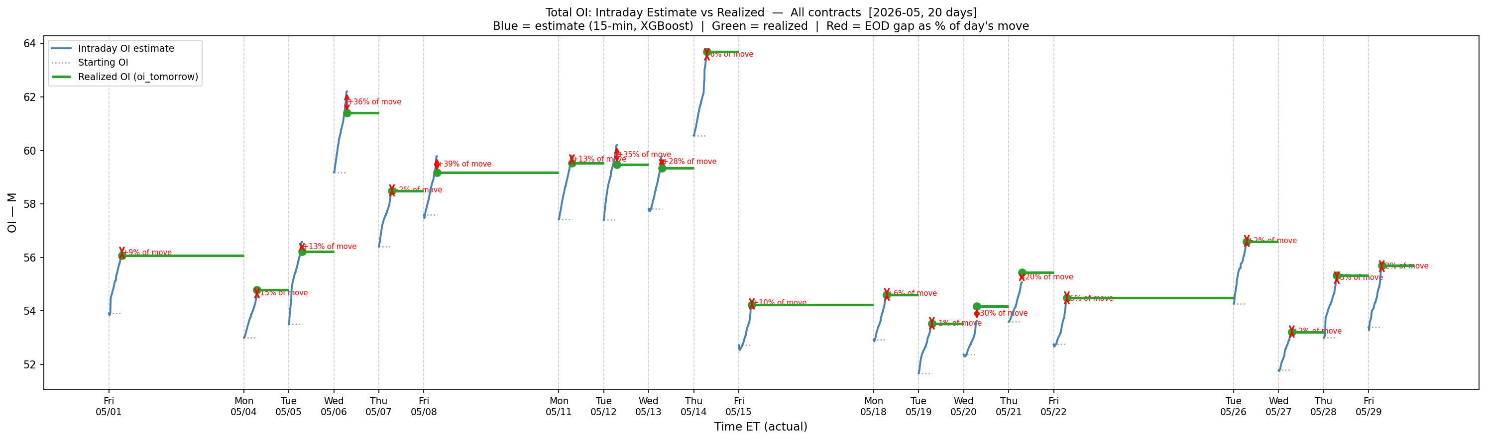
The chart above plots 20 consecutive trading days in May 2026. Each day shows the model's running estimate starting from the previous session's settled OI and updating continuously as new snapshots arrive through the session. The green marker at the close shows where OI actually settled. The red arrows show the size and direction of the terminal error.
On most days the estimate is close: within a fraction of a percent of the day's net OI move. The model typically identifies both the direction and the approximate magnitude of the positioning change well before the session ends, often within the first hour of trading as volume patterns establish themselves.
The outlier days (where the red arrows are longest) cluster in the first two weeks of May 2026, a period characterised by elevated macro uncertainty and above-average volatility. The pattern is consistent: on those days the model overshoots, expecting more OI accumulation than actually materialises. This is interpretable: in high-volatility regimes, traders close positions at higher rates than the model expects, because the training data represents a broad range of market conditions where the average participant behaviour is less defensively biased than during acute stress episodes.
The gap between what the model expects and what actually occurs is itself informative. Systematic and persistent model overshooting (the model predicting more opening flow than materialises) has historically coincided with elevated risk aversion and position reduction across the market. The estimation error is not just noise; under the right conditions it reflects something real and observable about the market's current disposition.
A Note on the Chart's Data Sources
Each element of the chart draws from a distinct snapshot in time, which is worth being explicit about. The grey dotted starting OI line is read from the last pre-market snapshot available before 09:30. That is typically a file stamped around 03:00 ET, which already reflects the previous night's settled, cleared OI. The green realised OI line is read from the following day's equivalent pre-market file. The blue intraday estimate starts anchored to that same pre-market OI value and then updates continuously using 15-minute session snapshots from 09:30 through 16:00.
An observant reader will notice that the aggregate total shown by the green line at the close of one session does not always match the grey dotted line at the open of the next. This is not a data inconsistency. For any individual contract, the two values are drawn from the same file and are identical. The aggregate total differs between sessions because the universe of active contracts changes day to day: the dataset includes only contracts that met a minimum activity threshold on each specific session. That set shifts as contracts near expiry, roll off, or become newly active. The gap is most pronounced across weekends and around monthly expiry, when a large cohort of contracts exits the active universe entirely. The model's per-contract accuracy metrics are unaffected by this aggregation effect. All training, evaluation, and error measurement is done at the individual contract level.
Deployment: Inference in the Browser, Updated Every 15 Minutes
A model that runs overnight is useful for research. A model that updates continuously throughout the session is useful for trading. The production deployment of this system runs inference entirely client-side: the trained model is hosted on cloud edge storage and loaded once per session, with subsequent predictions computed locally in the browser as each new snapshot arrives.
This architecture has meaningful practical advantages. Latency is minimal: there is no round-trip to a prediction server for each update. The system degrades gracefully if connectivity is interrupted, continuing to operate from the last loaded model. And because inference runs in the user's browser rather than on a centralised server, there is no prediction infrastructure to maintain or scale as usage grows.
The 15-minute delay inherent in the data source means estimates are always slightly lagged relative to the true current state. That is a constraint of the underlying data, not of the model. Within that constraint, the system provides the most current available estimate of intraday OI throughout the trading session, updated as frequently as the data allows.
The Data Market: What Proprietary Services Offer and Where the Gaps Are
A number of commercial tools have emerged in recent years claiming to give traders a real-time or near-real-time view of options positioning. Some of them explicitly argue that any gamma exposure tool which does not source a specific category of data directly from the exchange is fundamentally flawed. That is a strong claim, and it deserves a careful look.
What These Services Actually Buy
The dataset at the centre of these claims is the Open-Close Volume Summary published by Cboe. Unlike standard options volume data, this feed tags each trade with a directional flag showing whether the transaction was an opening trade (creating a new position) or a closing trade (unwinding one). The feed also categorises each trade by participant type: Market Maker, Broker-Dealer, Professional Customer, or retail Customer. It also applies a size filter, treating orders below roughly 100 contracts as retail and orders above 199 contracts as institutional.
This is genuinely useful information. If you can see that retail participants are aggressively opening calls at a particular strike while institutions are closing puts, that tells you something meaningful about where future hedging pressure will concentrate. The directional decomposition (opening versus closing, by actor) is a step beyond raw volume that aggregated data cannot provide.
So why the caveats?
The 50/50 Structure of Options Markets
To understand the limitations of actor-segmented data, it helps to understand the fundamental structure of options trading. Market makers are the liquidity backbone of the options market: they are present on one side of virtually every transaction, providing the bid or ask that allows a trade to occur at all. As a result of this structural role, the aggregate volume breakdown is approximately symmetric: market makers account for roughly 50% of all contracts traded, with retail and institutional customers together accounting for the other 50%.
Because a market maker is on one side of almost every trade, total consolidated open interest at any strike is (in aggregate) approximately half market maker positions and half customer positions: by structural necessity, not coincidence. Any tool that reports total OI is, implicitly, already capturing both sides of this relationship.
This creates an important logical constraint for claims about "market maker OI" as a uniquely valuable signal: if market makers are always on one side of the trade, their aggregate positioning is largely a mirror image of the customer side. Knowing one tells you the other. The genuinely new information in actor-segmented data is not whose position is what, but which direction (opening or closing) each side is moving. That is the actual signal.
The SPX Special Case
There is one instrument where the Cboe data is genuinely comprehensive: SPX index options. Because SPX options trade exclusively on Cboe exchanges, Cboe's Open-Close feed captures 100% of SPX volume with no fragmentation across other venues. For tools built specifically around SPX (which is where several prominent commercial products are focused) the exchange coverage limitation does not apply.
For equity options and ETFs, the picture is different. Options on names like the major equity ETFs or large-cap individual stocks trade across multiple competing exchanges. Cboe's data captures roughly 25 to 40% of that volume. A provider claiming to show you the full actor breakdown of open interest for equity options based solely on Cboe data is working with less than half the picture.
| Instrument type | Cboe exchange coverage | Open-Close data completeness |
|---|---|---|
| SPX index options | ~100% | Complete: all volume on Cboe exchanges |
| Major ETF options | ~25 to 40% | Partial: majority of volume on competing exchanges |
| Equity options | ~25 to 40% | Partial: fragmented across Nasdaq, NYSE, MIAX |
The Delay Problem
Commercial access to the Cboe Open-Close feed comes in three tiers. The end-of-day summary (which most subscribers use) is delivered overnight, after midnight U.S. Eastern, per Cboe's product documentation. It is useful for next-morning analysis, not for intraday decisions. The intraday versions disseminate data in 10-minute or 1-minute interval files, delivered minutes after each interval closes via SFTP or Snowflake. There is no fixed published delay figure; in practice the effective latency is the interval length plus file delivery, and subscribers have reported delivery running longer than the nominal few minutes at times. Even at its best, this is batch-file delivery, not a streaming feed: the open/close classification is compiled after each interval closes rather than at matching-engine speed.
There is no sub-minute, true real-time version of this data available at any commercial price point. Firms that have attempted to reconstruct real-time actor-segmented flow from raw exchange feeds have done so through co-location infrastructure reportedly costing in the range of $20,000 to $50,000 per month, using proprietary algorithms to infer open/close intent from order characteristics. That is in essence a more expensive version of the same inference problem our model solves.
For completeness, there is one tier below the summaries: Cboe's Enhanced Trade-by-Trade Execution Detail dataset, the individual execution records the Open-Close files are aggregated from. Each print carries its buy/sell and open/close markers, participant capacity, and the NBBO at the moment of execution. Execution IDs link the legs of complex trades (C1 only so far, delivered T+1, history back to October 2019). It is not a dashboard input and it is not real-time; its value is different: per-trade ground truth, which makes it the natural dataset for training and validating classification models rather than for displaying positioning.
How Our Approach Compares
Our model operates on 15-minute delayed consolidated snapshot data. For SPX, Cboe's 1-minute intraday tier (delivered minutes after each interval closes) is genuinely the lower-latency source, and we will not pretend otherwise. The honest comparison is not about latency: it is coverage, scope, and cost. On one side: actor-segmented opening/closing volume on Cboe exchanges only, at a meaningful subscription price per instrument scope. On the other: a full-market consolidated OI estimate with a measured error rate, across every instrument the snapshot feed covers, at no marginal data cost.
| Dimension | Cboe Open-Close (standard tier) | Our intraday OI model |
|---|---|---|
| Intraday latency | 1-min interval files, delivered minutes after each interval closes (intraday tier) | 15-minute delayed snapshot feed |
| Market coverage | Cboe exchanges only (25 to 100% depending on instrument) | Full consolidated OI across all exchanges |
| SPX specifically | Complete (100% Cboe) | Complete (full consolidated) |
| Estimation error | None (exact, for captured volume) | ~12% on snapshot classification; <15% of daily OI move at EOD |
| Ongoing data cost | Subscription priced per exchange and scope; intraday tiers cost more than EOD | No ongoing data cost beyond existing snapshot feed |
| Historical depth | Multi-year, all-symbol backfills quoted at institutional price levels | Built from accumulated snapshot archive |
The honest summary is that actor-segmented open-close data and aggregate intraday OI estimation are measuring related but different things. The Cboe product tells you the directional intent of identifiable participant categories. That is valuable, and on its intraday tier it arrives with lower latency than our snapshot feed. But it does so with exchange-limited coverage outside SPX and at a subscription cost that scales with scope. Our model estimates total consolidated OI continuously with a measured error margin, covers all exchanges equally, and operates at no marginal cost per instrument added.
For SPX specifically (where Cboe coverage is complete) the two approaches are most directly comparable, and the question of which provides more actionable information depends on the use case. For everything outside pure SPX, the coverage argument runs strongly in favour of consolidated estimation.
The broader point about claims that only actor-segmented data from the exchange constitutes "real" gamma information deserves scrutiny. Given that market makers are structurally on one side of approximately half of all trades, aggregate open interest already encodes the combined positioning of all participants. The additional value of actor segmentation lies in the directional decomposition (opening versus closing pressure by participant type) which is meaningful, but which does not negate the value of total consolidated OI as the foundation for gamma exposure analysis.
Limitations and What Comes Next
This is a first-generation system, and it has known limitations worth being explicit about.
Binary framing is a simplification. Classifying each unit of volume as purely opening or purely closing is a useful approximation, but options volume includes more nuanced flow (spread trades, rolls, exercises approaching expiry) that does not map cleanly into either category. Future iterations could explore richer target formulations that account for these transaction types explicitly.
The model does not observe order flow. The true signal of opening versus closing intent is embedded in order flow data: whether trades were buyer- or seller-initiated, at what price relative to the bid-ask midpoint. We infer intent from aggregate outcomes. Access to tick-level flow data would substantially change the problem framing and likely improve performance further.
Regime adaptation is limited. The model was trained across a range of market conditions, but sustained regime shifts could degrade its calibration over time. Periodic retraining as new data accumulates is part of the production workflow, but it is not a complete adaptive solution.
Equity coverage is currently selective. The zero-shot transfer results are encouraging but were evaluated on a set of large-cap names with liquid options markets. Extension to smaller, less-liquid underlyings (where OI dynamics may differ structurally) is an open question that requires further testing.
0DTE as an explicit indicator. One natural extension that falls directly out of the existing data is a real-time 0DTE volume share: the percentage of each session's total options volume attributable to same-day-expiry contracts, updated every 15 minutes alongside the OI estimate. The model already handles 0DTE contracts separately (by construction their contribution to overnight OI is zero) but surfacing the 0DTE share explicitly would make a hidden dynamic visible. On high-0DTE days, a large intraday OI build on the estimate curve can collapse nearly to zero by the close, not because the model failed but because the underlying volume was speculative and ephemeral. Displaying the 0DTE fraction alongside the OI trajectory would provide immediate context for that behaviour, and would double as an independent regime indicator: elevated 0DTE participation compresses the useful information content of aggregate OI and shifts the character of intraday dealer hedging in ways the gamma exposure framework does not fully capture on its own.
Conclusion
The one-day lag in official open interest reporting has been accepted as a structural feature of equity options markets. We treated it as a problem worth solving.
The result is a machine learning system that estimates intraday open interest in real time from 15-minute volume snapshots, trained jointly across a set of index and ETF option products, and deployable immediately to equity underlyings without retraining. The system achieves meaningful improvements over single-instrument baselines, and (more importantly) demonstrates that the underlying dynamics of OI formation are sufficiently consistent across instruments to support a genuinely universal model.
The practical implication is a real-time gamma exposure view that updates continuously through the session, rather than one that resets each morning from the previous day's data. That represents a material improvement in the quality and timeliness of available information for participants who rely on the gamma map to interpret intraday price behaviour, size positions, or manage risk.
The research is ongoing. The results presented here represent a stable, validated system. Not a final answer. The gap between what is currently achievable and what a fully adaptive, order-flow-aware system might deliver remains substantial. Closing it is the next challenge.
Explore the Live Gamma Exposure Dashboard
The model described in this article powers our real-time gamma exposure tool. See intraday OI estimates updated every 15 minutes throughout the session across indices, ETFs, and major equities.
View Live Dashboard What Is Gamma Exposure?